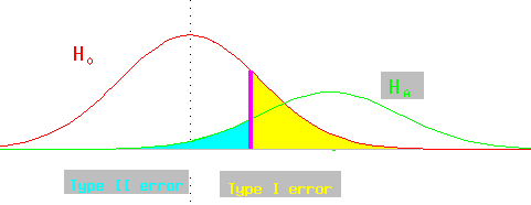
Type II error
A type II error occurs when one rejects the alternative hypothesis (fails to
reject the null hypothesis) when the alternative hypothesis is true. The
probability of a type II error is denoted by *beta*. One cannot evaluate the
probability of a type II error when the alternative hypothesis is of the
form µ > 180, but often the alternative hypothesis is a competing
hypothesis of the form: the mean of the alternative population is 300 with
a standard deviation of 30, in which case one can calculate the probability of
a type II error.
Examples:
If men predisposed to heart disease have a mean cholesterol level of 300
with a standard deviation of 30, but only men with a cholesterol level over
225 are diagnosed as predisposed to heart disease, what is the probability of
a type II error (the null hypothesis is that a person is not predisposed to
heart disease).
z=(225-300)/30=-2.5 which corresponds to a tail area of .0062, which is the
probability of a type II error (*beta*).
If men predisposed to heart disease have a mean cholesterol level of 300
with a standard deviation of 30, above what cholesterol
level should you diagnose men as predisposed to heart disease if you want the
probability of a type II error to be 1%? (The null hypothesis is that a
person is not predisposed to heart disease.)
1% in the tail corresponds to a z-score of 2.33 (or -2.33); -2.33 × 30 =
-70; 300 - 70 = 230.
Conditional and absolute
probabilities
It is useful to distinguish between the probability that a healthy person is
dignosed as diseased, and the probability that a person is healthy and
diagnosed as diseased. The former may be rephrased as given that a person is
healthy, the probability that he is diagnosed as diseased; or the probability
that a person is diseased, conditioned on that he is healthy. The latter refers
to the probability that a randomly chosen person is both healthy and diagnosed
as diseased. Probabilities of type I and II error refer to the conditional
probabilities. A technique for solving Bayes
rule problems may be useful in this context.
Examples:
If the cholesterol level of healthy men is normally distributed with a mean of
180 and a standard deviation of 20, but men predisposed to heart disease have
a mean cholesterol level of 300 with a standard deviation of 30, and the
cholesterol level 225 is used to demarcate healthy from prediposed men;
what fration of the population are healthy and diagnosed as predisposed? what fraction of the population are predisposed and diagnosed as healthy? Assume
90% of the population are healthy (hence 10% predisposed).
Let A designate healthy, B designate predisposed, C designate cholesterol level below 225, D designate cholesterol level above 225. P(D|A) = .0122, the
probability of a type I error calculated above. Hence P(AD)=P(D|A)P(A)=.0122
× .9 = .0110. P(C|B) = .0062, the probability of a type II error calculated above. Hence P(CD)=P(C|B)P(B)=.0062 × .1 = .00062.
A problem requiring Bayes rule or the technique referenced above, is what is the probability that someone with a cholesterol level over 225 is predisposed to heart disease, i.e., P(B|D)=? This is P(BD)/P(D) by the definition of conditional probability. P(BD)=P(D|B)P(B). For P(D|B) we calculate the z-score (225-300)/30 = -2.5, the relevant tail area is .9938 for the heavier people; .9938 × .1 = .09938. P(D) = P(AD) + P(BD) = .0110 + .09938 = .10038 (the summands were calculated above). Inserting this into the definition of conditional probability we have .09938/.10038 = .90034 = P(B|D).
Remarks
If there is a diagnostic value demarcating the choice of two means, moving it
to decrease type I error will increase type II error (and vice-versa).

The power of a test is (1-*beta*), the probability of choosing the alternative hypothesis when the alternative hypothesis is correct.
The effect of changing a diagnostic cutoff can be simulated.
Applets: An applet by R. Todd Ogden also illustrates the relative magnitudes of type I and II error (and can be used to contrast one versus two tailed tests). [To interpret with our discussion of type I and II error, use n=1 and a one tailed test; alpha is shaded in red and beta is the unshaded portion of the blue curve. Because the applet uses the z-score rather than the raw data, it may be confusing to you. The allignment is also off a little.]
Competencies: Assume that the weights of genuine coins are normally distributed with a mean of 480 grains and a standard deviation of 5 grains, and the weights of counterfeit coins are normally distributed with a mean of 465 grains and a standard d
eviation of 7 grains. Assume also that 90% of coins are genuine, hence 10% are counterfeit.
What is the probability that a randomly chosen genuine coin weighs more than 475 grains?
What is the probability that a randomly chosen counterfeit coin weighs more than 475 grains?
What is the probability that a randomly chosen coin weighs more than 475 grains and is genuine?
What is the probability that a randomly chosen coin weighs more than 475 grains and is counterfeit?
What is the probability that a randomly chosen coin which weighs more than 475 grains is genuine?
Reflection: How can one address the problem of minimizing total error (Type I and Type II together)?