Consider the simple two-player game I call the End Game. The game board consists of a list of N arbitrary integers, where N is even. Each player begins with a score of 0. The players alternate choosing a number from the list and adding its value to their score. The only requirement is that players can only choose one of the numbers on the ends of the list. When no numbers remain, the game is over. The player with the larger score wins. The difference between the scores does not matter.
For example, consider this starting position:
-1 3 9 4
The first player can choose either -1 or 4. Suppose he chooses 4. The new position is:
-1 3 9
The second player can choose either -1 or 9. Suppose she chooses 9. The first player can now choose either of the remaining numbers. When he chooses 3, the second player must take -1.
With all numbers chosen, we look at the player's sums. The first player has 4 + 3 = 7, and the second player has 9 + (-1) = 8. The second player wins.
Suppose that the players reverse roles. The game might proceed as follows: she takes -1, he takes 4, she takes 9, and he takes 3. The second player -- this time moving first -- wins again!
Your opening exercise is to play this game several times against different players. You will play two games against each opponent, with each of you going first once.
Try to find a strategy that works for you, and record it. Don't share your strategy with your opponents yet! Let them try to figure out a good strategy on their own.
... much fun ensues in the first round ...
You should have some strategy for playing by now, though it may not work all the time or you may not implement it correctly every time. It may not even be very good!
Now you will play against two more opponents. Use your strategy, and see how well it works on the new game positions.
... more fun ensues ...
Today's .zip file contains a simple Java program to generate random game boards and a file containing all the boards we used today, plus a few more!
How well did your strategy work? Does it win when possible? Is it simple to use? Is it simple to explain?
It turns out that the player who moves first can always earn at least a tie. This requires what we call a non-losing strategy. Indeed, there are several different non-losing algorithms for this game. Let's consider several different ways to design or discover algorithms for playing the game, and see what we can learn from them.
First of all, we can characterize some strategies in terms of the kinds of moves they make.
You could combine two strategies, say, choosing randomly or greedily until the list gets short enough that you can plan ahead effectively. This is called a hybrid strategy. Introselect, mentioned in the Wikipedia article about quickselect, is a hybrid algorithm.
Random and greedy algorithms are often quite useful, depending on the type of problem we are solving. We will encounter them again throughout the course.
But we can also characterize strategies in terms of the way we develop the algorithm. In this regard, there are three high-level approaches to designing an algorithm:
Let's consider each in turn.
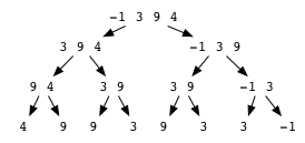
Each move changes the game board into a sub-list of the original. It also changes who is "on move".
We could create a tree of all the possibilities, and then use that tree to help us choose the better move. Such a tree is called a game tree, and we can explore it with recursive calls and backtracking.

Let's assume that our opponent play optimally. How can we find the best move?
When we try to evaluate a position L the tree, we need to know what the loser will score from each of its sub-positions, Ll and Lr. The opponent will be on move in those positions, and we assume that she will play optimally. We want to maximize the score we receive by choosing one of L[1] or L[n].
The rule for choosing left or right is thus:
    If L[1]+loser(Ll) >= L[n]+loser(Lr),
       then choose left
       otherwise, choose right
Now we need a way to compute loser(L). If the length of L is 2, then the job is easy: loser(L) is the smaller of the two. If L has more than two elements, then the losing value is what's leftover after the player on the move makes the optimal choice:
    If not, choose left or right using the above rule.
       If the move is left,
          loser(L) is sum(L) - (L[1] + loser(Ll)).
       If the move is right,
          loser(L) is sum(L) - (L[n] + loser(Lr)).
That sound complicated, but computers are pretty good at this sort of computation. Let's try it out for the initial position of -1 3 9 4...
[ ... trace on the above diagram ... ]
Notice that the definition of loser(L) is inductive. The length-two case is the base case, and the other is the inductive case.
Decomposing the problem in this way and solving sub-parts first is an example of a common algorithm design pattern known as divide and conquer. We will consider a number of forms of divide-and-conquer throughout the course.
This algorithm works. It will never lose for the player moving first. But how good is it?
Notice that our tree contains one line of length N, two of length N-1, four of length N-2, ... and 2n-2 of length 2, at which the choice becomes obvious. Some of these smaller boards are repeated, but they will be considered multiple times by the algorithm.
Thus, this solution is exponential in the length N. If this was your strategy earlier, you probably ran into some problems when the list of numbers went from size 4 to size 10!
We can implement this algorithm in a program straightforwardly using recursion. But such an implementation will recompute many of the loser sums. Look at that tree again... We can implement the same idea more efficiently using a technique known as recursive backtracking. Recursive backtracking is a common design pattern in two-person games with "complete information".
Can we avoid the recursive calls altogether, and thus perhaps avoid some of the exponential load of the algorithm?
Why not come at this problem from the other direction? We can compute best moves for all tables of length 2, and then for all tables of length, and so on, until we have computed the best move for the starting table of length N. We can compute each value once, store the result in a table, and then re-use it whenever we need it later. No recursive calls!
Once we have the table with the answers for all possible sub-lines of L, smallest first, making moves is an O(1) look-up.
(This introduces another dimension into our design space: batch computing time versus distributed computing time. What if we don't have time to do the table-building computation up front?)
The algorithm looks something like this:
    for size := 2 to n
        for left := 1 to (n-size+1)
            1. compute and store sum  [left, left+size-1]
            2. compute and store move [left, left+size-1]
            3. compute and store loser[left, left+size-1]
Computing the sum of a sub-line is trivial. Computing the correct move for a sub-line is done in terms solely of the sub-line and previously-computed loser values:
    if size = 2
       then if L[left] > L[left+1]
               then return "left"
               else return "right"
       else if L[left] + loser[left+1, left+size-1]
                  > L[left+size-1] + loser[left, left+size-2]
               then return "left"
               else return "right"
Finally, computing the loser sum for a sub-line is done in terms of this iteration's sum and move and the previous iteration's loser values:
    if size = 2
       then return min( L[left], L[left+1] )
       else if move[left, left+size-1] = "left"
               then return sum[left, left+size-1]
                             - (L[left] + loser[left+1, left+size-1])
               else return sum[left, left+size-1]
                             - (L[left+size-1] + loser[left, left+size-2])
Again, let's try this out for the initial position of -1 3 9 4...
[ ... trace on the above diagram ... ]
This is an example of the technique known as dynamic programming, in which we compute and store the solutions to sub-problems so that we never have to compute them more than once each.
How does this algorithm compare to our top-down algorithm above?
(But this algorithm can also generate optimal play in variations of the game where the number of points a player scores matters, whereas the top-down algorithm does not.)
Can we do as well or better with a simpler algorithm?
The idea here is to use knowledge:
We don't need to consider all possible states of the game if we can force play into a smaller set of scenarios...
Look for an invariant property controlled by one of the players. In the End Game, we'd like an invariant property controlled by the player who moves first.
[ ... fill in the blank ... ]
... Player 1 can turn it into a game of evens versus odds!
... sometimes we can find an invariant solution directly.
... sometimes it is helpful to work through the approaches in order.
... exposure, familiarity, experience.
The result: off by two. Why? Students who entered the room late, or unclear instructions, or incorrect execution.
... but: a useful first example: simple enough to grasp the parts, complex enough to raise lots of interesting questions, drawing on your knowledge and past experience.
your questions
  - answered a few directly
  - if you want that, or more, let me know
  - some recurring questions and issues

how can the swaps to create the partitions?
  - work through algorithms on small examples,
    to see if you can see the pattern
  * work an example (or show basic idea) in class

terms
  - in-place algorithm     more space to store the items
  - stable vs unstable     does the order of values change?

big question
  - how do we select a good pivot?
  - won't more complex pivot selection algorithms add enough
    overhead to negate the advantage of a better pivot?

median of three
   - use median of 1st, mid, last items as pivot
   - "Compared to picking the pivot randomly:
      - It ensures that one common case (fully sorted data)
        remains optimal.
      - It's more difficult to manipulate into giving the
        worst case.
      - A PRNG is often relatively slow."

median of medians
   - create five partitions, find median of each
   - use median of those five items as pivot
   - more overhead...  how can it improve enough?


"median-of-3 killer"
   - an example that causes the algorithm to have its worst case

hybrid algorithms: knowledge, complexity, performance