Measures of location
Often it is not possible to list all the data or draw a histogram; it would be
nice to have one number which best represents a data set. Often where the data
lies is of interest, for which purpose a measure of location is useful. There
are several measures of location, which we shall illustrate with the data sets
A={2, 9, 5, 3, 8}, B={1, 4, 7, 3, 9, 2}, and the
weights of students of a previous lesson.
The minimum is the smallest value in a data set. It is often useful to put
data
in rank order when studying it, in which case A would be represented as
{2, 3, 5, 8, 9} and B as {1, 2, 3, 4, 7, 9}, and the
rank order of the weights was given before.
From these rank order listings, it is immediate that the minimum of A is 2,
the
minimum of B is 1, and the minimum of the weights is 105.
The maximum is the largest datum in a data set. From the above rank order
listings, it is immediate that the maximum of A is 9, the maximum of B is 9,
and the maximum of the weights is 235.
The midrange is the middle value in the sense that it is halfway between
the maximum and minimum. It is computed as (maximum+minimum)/2. The midrange
for data set A is (9+2)/2=5.5, the midrange for data set B is (9+1)/2=5, the
midrange for the weights is (235+105)/2=170. The midrange is easy to
calculate,
but because it is defined by the two extreme data, it may not be representative
of where most of the data lie. The midrange is seldom used, one text said that it should be defined solely so the student will not confuse its definition with that of the median.
The median is the middle value in the sense that half the data are above it,
and
half the data are below it. If there are an odd number of data points, the
median is the middle value, e.g., 5 for data set A. If there are an even
number
of data, the median is half way between the two middle values, e.g.,
(3+4)/2=3.5 for data set B and (155+155)/2=155 for the weights. When finding
the median, make sure the data are in rank order, and each value has been
listed as often as it occurs. The median is perhaps the best indicator of
where the
data lies, being truly amid the data values. Some
comments on the median by Stephen Jay Gould may be of interest.
The mean (which is represented as an overscored x which is pronounced x-bar)
is calculated by adding up all the data values and dividing by the
number of data (usually denoted by n). This formula can be concisely
represented using summation notation. For data set
A the mean is (2+3+5+8+9)/5=5.4, for data set B the mean is
(1+2+3+4+7+9)/6=4.33, for the weights the mean is
(105+110+112+113+120+125+125+130+...+235)/30=153.43. The mean reflects all
the
data, hence can be significantly impacted by extreme values; but is widely used because it can be algebraically manipulated and works
well with other statistics.
If a data set is symmetric, the mean is equal to the median, which is equal
to the midrange.
As the median divides a data set in half,the quartiles divide the data set
into fourths. Hence the second quartile, denoted Q2, is the median. However,
there are several definitions for the first and third quartile which result in
different values when applied to some data sets. Heuristically, the first quartile is the median of the lower half of the data and the third quartile is the median of the upper half of the data, but if there are an odd number of data, the question of whether to include or exclude the middle datum with/from the upper and lower halfs of the data arises. For the weights of the students, there is an even number of
data points (30) and no datum is at the median (actually, three students
weigh 155, but we consider two of them as in the lower half of the data and one
as in the upper half to get 15 individuals in the lower half and 15 in the
upper half). Thus taking the respective medians, Q1 = 130 and Q3 = 175.
Q2 is of course always equal
to the median (in this case 155). The first quartile is the 25th percentile and the third quartile is the 75th percentile; the formula to compute percentiles (presented later) can be used to calculate quartiles.
[Although the manual suggests the that the TI-83 includes the median in both
the lower half and upper half of the data for calculating Q1 and Q3, respectively, it actually excludes (instead of
includes) the median.]
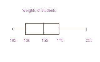
A single number is often not adequate to convey where the data in a data set
lie. However, giving the minimum, three quartiles, and maximum provides
extensive information about the distribution of the data. These five
statistics of a data set are displayed pictorially in a box-and-whisker plot (boxplot). The
first and third quartiles are at the ends of the box, the median is indicated
with a vertical
line in the box, and the maximum and minimum are at the ends of the whiskers. A
boxplot for
the weights is depicted below. (If the minimum or maximum are very extreme ("outliers"), the whiskers may not extend to the minimum and maximum, but they will be identified with asterisks in the box-and-whisker plot.)
N.B.:
especially from looking at boxplots, one can see that in general quartiles are
not symmetric, i.e., Q2-Q1 is not equal to Q3-Q2.
Competencies: For the data set {2 5 9 4 6 7 6 8 8}, calculate the mean,
median, midrange, maximum, minimum, Q1, and Q3.
Reflection: For the above data set, which of the above statistics best
describes where the data is?
Challenge: When will the mean, median, and midrange be equal? When
will the maximum, minimum, Q1, Q3, and median be equal?
return to index
Questions?
July 2007