Frequency distributions
With cartons of eggs, we can count the number of cartons which have one, two,
or three (etc.) broken eggs; there cannot be a fractional number of broken eggs
in a carton. Such data is called discrete -- every datum takes on one of a few
specified values. When measuring height, any real number is a possible
value; am I 6'2", 6'1.9375", or 6'1.93814" tall? It is really more
appropriate to
describe my height as being in the interval 6'1.5" - 6'2.5" than as equal to
6'2". Data sets which can take on any value in a continuum are called
continuous. With discrete distribution you can have, e.g, exactly two eggs,
but with continuous distributions nobody is , e.g., exactly two metres tall.
Hence with discrete distributions strict versus weak inequalities are
important, but with continuous distributions it does not matter whether
inequalities are strict or weak.
We have constructed histograms so that the height of each bar is the number of
data in each class. We can rescale our axis so that the total area of the
histogram is equal to one, in which case the area of a rectangle will be the
proportion of the data set which is in the class. This is easily generalized
for any curve with the total area under the curve equal to one: The
proportion of a data set in an interval is equal to the area under the curve
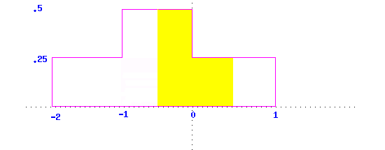
above that interval. In the following graph we can calculate that the relative
frequency of data in the interval (-.5, .5) is .375 (the area of the yellow
region) by using the area formula for rectangles.

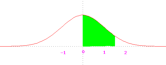
If the graph is not rectilinear, more sophisticated techniques are necessary,
but it can be shown that the area of the shaded region in the following
graph is 0.43.

return to index
Questions?

